A decent introduction to Gradient Descent in Python

Gradient Descent is a fundamental element in today’s machine learning algorithms. We use Gradient Descent to update the parameters of a machine learning model and try to optimize it by that. The clue is that the model updates those parameters on its own. This leads to the model making better predictions.

In the following article we’ll dive into Gradient Descent, and I’ll explain it with the help of an example scenario which we’ll solve using Supervised Learning and Python. We won’t use any ML framework like PyTorch or TensorFlow for that. The complete source code is available at GitHub.

Supervised Learning

Let’s have a look on Wikipedia’s definition for Supervised Learning.

Supervised learning is the machine learning task of learning a function that maps an input to an output based on example input-output pairs. (Source: Wikipedia)

Sounds confusing, but it’s quite easy actually. An example might be good.

Let’s say you want to make a computer tell you whether a photo is the one of a cat or not. Before the computer is able to tell you whether it’s a cat or not, you have to teach the computer how a photo of a cat looks like. For that, you feed the computer with many photos (input) and the information whether the photo is that one of a cat or not (output). This process is called training phase.

When the training phase is completed, you can show your computer a photo of a cat that it has not seen before, and it tells you whether it’s the one of a cat or not. Artificial Intelligence, amazing! For that, your computer uses the function that it just learned before.

This cat example is a classification problem. Classification is the task of predicting a discrete class label (“cat” and “no cat”). The other type of problem is called Regression, which is the task of predicting a numerical or continuous value. The example below is such a Regression problem.

The Scenario

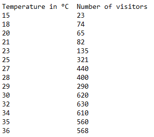
Imagine we’re the owner of an amusement park. For organizational reasons we want to know, or at least predict, the number of visitors for the next day. Fortunately, we took some notes about the number of visitors based on the weather in the last season.

Regarding Wikipedia’s definition of Supervised Learning those values are the so-called “example input-output pairs”. The temperatures are the “input” and the number of visitors are the “output”.

For example, when there was 30 °C outside our park had 620 visitors. These notes are the training data for our ML model. The values in the left column are called features. The ones in the right column are called labels.

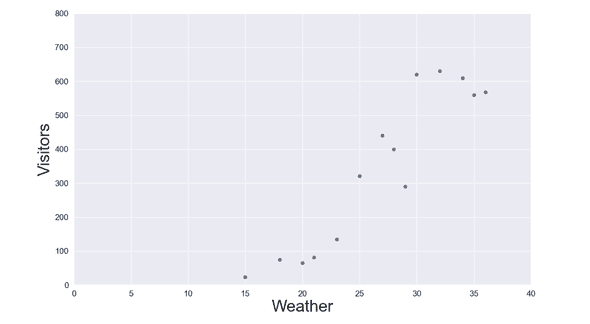
Last but not least the noted data put in a beautiful diagram.

Back to our question. How many visitors can we expect to see in our park tomorrow when know that there will be 33 °C at this day? As you can see we have no information about the number of visitors for 33 °C in our table. We have to predict the value. Let’s do it!

Linear Regression

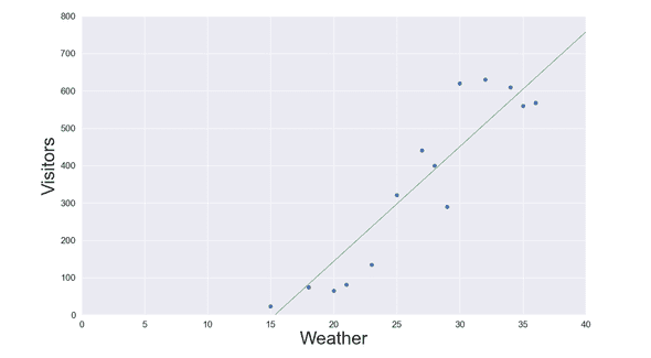
Linear regression helps us find the “best fitting straight line” that we can place inside the data in of diagram. When we found this line, we can use it to predict other values that are not part of our records, like tomorrow’s number of visitors when there are 33 °C outside.

You might remember from school that a linear function is described as:

• y is the output (visitors) also known as f(x)
• m is the slope
• x is the explanatory variable (weather)
• b is the bias

This equation might be also familiar to you with some other variable names. Using this equation, which represents our line, we can predict the output (y) for any given input (x) later on.

In our scenario we’d like to predict the number of visitors (y) when there are 33 °C (x) outside, so it is f(33) = y = m * 33 + b.

For this, we have to choose values for m and b wisely. Fortunately, the computer will do this for us. They are the learnable parameters inside the model.

Well, now that we know this equation is used to predict values. Let’s implement this one in Python:

# The model's output (prediction)
def predict(X, w, b):
    return X * w + b

Note that we changed the name of the variable x to w, which means weight. Our goal is that this predict() function tells us the output for any given input variable X. For that, we need to assign values to w and b.

Before we find these values let’s look for a way to measure the quality of our new function. A so-called loss function can do this for us.

Loss Function

The loss function measures how far a model’s predictions are from its label. In other words: it determines how good or bad our model is.

Since we’re using linear regression, we don’t have to invent our own loss function. There is already one we can use. This one is called mean squared error (MSE).

The function includes four variables n, i, y' and y:

• n is the number of input-output pairs we have (14)
• i is the index for the current pair from our training data we’re looking at
• y' is the predicted value from our model which we’ll get from the predict() we declared at the beginning
• y is the actual output value that we got from our training data label

For each value from our training data this function calculates the difference between the label and the predicted value from predict() and squares the result. All these results are summed up and at the end the mean is taken.

Now we can use the loss function to determine how good or bad our model is. The smaller the output value of the function is the better is our model, because only few errors were made in this case. A high value implies a worse model on the other hand. So, our goal is to minimize its output because we want as few errors as possible.

Let’s implement the MSE in Python.

# Calculating the loss using MSE
def loss(X, Y, w, b):
    return np.mean((predict(X, w, b) - Y) ** 2)

Here we have four arguments:

• X is an Numpy array containing temperaturs (features)
• Y is an Numpy array containing number of visitors (labels)

w and b are used for the predict() function, whose output is equivalent to y in the MSE equation. Since X and Y are both Numpy Arrays the part (predict(X, w, b) - Y) ** 2 is executed for each single array element.

Now we are able to measure how good or bad our model is. Keep in mind that we try to find good fitting values for w and b inside predict().

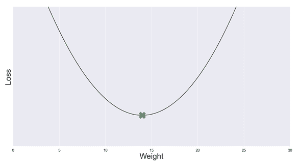
For now, let’s measure the loss of our model using the loss() function with some random numbers for the weight w. To make it easier we will set b = 0, so the prediction only depends on w.

You can see, the loss of model is the smallest when we set w = ~14. This position is also called minimum. Humans can identify this spot quite easily when they see the graph. A computer on the other hand can’t do so. Moreover, you don’t always know which number the weight w might be close to. What if the minimum had been at w = 3000? The scaling on the x-axis would be too small to identify the minimum visually.

So we need to find a way to tell the computer how to find this spot. For that, Gradient Descent is the right choice.

Gradient Descent

Gradient Descent is an algorithm for finding a local minimum of a function. In this case, we try to find the minimum of our loss function because at this position the model makes the best predictions.

In Gradient Descent we choose a random starting point in our graph. From this position we’ll take many steps towards the minimum. But how do we know in which direction (left or right) to go and how big a single step should be?

Gradient 1

For this, we use the so-called Gradient. The Gradient can actually have two meanings depending on the number of parameters of a function.

In both cases you can say that the Gradient of a function is calculated with the help of all its partial derivatives. But first, let’s talk about what the Gradient is.

One parameter: f(x)

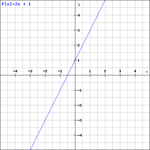
If we have a function like f(x) = 2x+1 that only depends on one parameter (x) the gradient is the degree of steepness of the graph at any given point, also known as slope. Time for an example.

This is the graph of the random chosen function f(x) = 2x+1.

Let’s calculate the Gradient for a given point. For this, we firstly calculate the partial derivatives with respect to x since this is our only parameter.

The result is 2, what is exactly the slope of the function f(x). Since it’s a linear function, the Gradient is equal to 2 at any given point x.

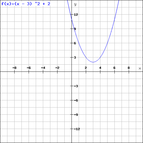
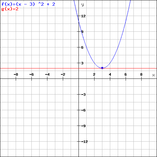
What if we have non-linear function like f(x) = (x-3)^2+2? In this case its graph looks like the following.

You might notice that this graph is similar to the one of our loss function above. Now, we calculate the Gradient for any point in this graph. Again, we firstly calculate the partial derivatives with respect to x since this is our only parameter.

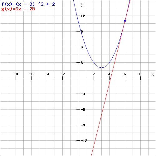
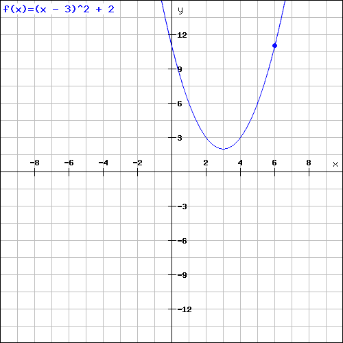
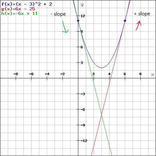
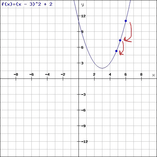
As you can see the slope is not the same for each point. Here, it depends on x. Let’s say we’re standing at x = 6 in our graph. What is the Gradient aka slope at this spot? In this case it’s 2*(6–3) = 6. The red line is the tangent with a slope of 6 at the given point x.

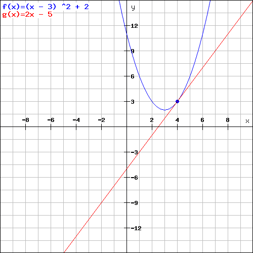
Another example. Let’s say we’re right at x = 4 in the same graph. Here, the Gradient aka slope is 2*(4-3) = 2.

The important thing here is that the Gradient decreases more and more the closer we’re at the graph’s minimum. Compare the slope of the upper two graphs at our example points. The second one has a smaller slope because the point is closer to the minimum.

At the graphs minimum, where x = 3, the Gradient is 0. There’s no slope at all at this position as the red tangent shows you.

So, in general we can say that the Gradient tells us whether we are far away from the graph’s minimum or not. The smaller the Gradient is the closer we are to the minimum.

Okay, but how does that help us? With the help of the Gradient we can minimize the output of our loss function. That’s what our goal is, we want to minimize the loss.

Let’s say the above graph is the course of our loss function where y is the loss and x is the weight. We want to find the value of x where y is the smallest since y is the loss, and we want a minimal loss in our model to make better predictions. In the scenario above, that would be at position x = 3.

But how do we find this spot x? That’s where the Gradient Descent algorithm comes into play.

Gradient 2

In Gradient Descent we set our x (weight) to a random initial value. Let’s say we set x = 6. That’s our starting point. In practice this value might be 0. Our function is the same as above.

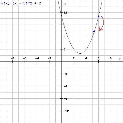
From there on, we calculate the Gradient for this given starting position x. Afterwards, we take a small step leftwards (because we want to reach the minimum) depending on the Gradient’s size.

How do we know whether we need to move to the left or to the right? In this case the Gradient is positive since there’s a positive slope at this position. So, we know that we have to go leftwards. If we are on a spot that is more left, we have to go rightwards because the slope is negative there.

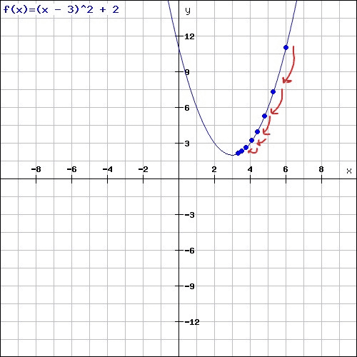
Let’s get back to the descent. Now we reached a new spot on our graph, which we again calculate the Gradient for. Then, we take another step leftwards. This time, however, the step we take is slightly smaller than the previous one, because the Gradient decreased as we come closer to the minimum.

We repeat this procedure multiple times until we reach, or at least are close to, the graph’s minimum.

The important thing here is, that the steps are getting smaller with each single step. That’s because our step size depends on the size of the Gradient (slope) at the given position, which is getting smaller and smaller the closer we are to the graph’s minimum. Just as you have seen above.

Actually, the step size does not only depend on the Gradient’s size. At our stating position (x = 6) the Gradient is also 6. Now imagine we go 6 steps leftwards. In this case we would miss the graph’s minimum and end up too far left. That’s why we have to go a certain proportion of the Gradient.

This proportion is also called learning rate. During each iteration of our Gradient Descent (when we take a single step) the algorithm multiplies the learning rate by the gradient. The resulting product is called the gradient step: gradient_step = lr * gradient. That’s the actual step we take leftwards.

The learning rate is a value we set on our own. We could use 0.001 for example. A too high learning rate might result in taking too large steps, and we might miss the minimum. If the learning rate is too small, we tend to not reaching the minimum in a given number of iterations.

This resulting gradient step in each iteration is then subtracted from our current weight, the x value: x = x - gradient_step. This way our weight becomes step by step closer to the target value: the value where the loss (y) is the smallest.

If the gradient_step is negative because the slope is negative, we add the gradient_step since minus and minus is plus and go rightwards accordingly.

Now let’s bring this all together and implement it in Python. Keep in mind that the graph’s x value is represented as the weight w in our codebase.

# The partial derivatives of "loss" with respect to w and b
def gradient(X, Y, w, b):
    w_gradient = 2 * np.mean((predict(X, w, 0) - Y) * X)
    return w_gradient

# Train the model using Gradient Descents algorithm
def train(X, Y, iterations, lr):
    w = 0 # Initial weight

    # Gradient Descents iterations
    for i in range(iterations):
        w_gradient = gradient(X, Y, w, 0)
        w -= w_gradient * lr
    return w

As I mentioned earlier, the Gradient is calculated using the partial derivatives of the function with respect to each single parameter. Our function in this case is the loss function (MSE). At the moment we’re just dealing with one parameter w. So, we calculate the partial derivative with respect to w. You can see the result in gradient(). This article might give you a better understanding of how the partial derivatives for the MSE are calculated.

Since we are just dealing with one parameter until now, we pass 0 for b when we call predict() in our gradient() function. We’ll fix this now.

Two parameters: f(x,y)

Until now, we assumed that our model only depends on one parameter x, also known as weight w. But that’s not the truth actually. If we take a look at the predict() function we can see that its output for a given value X depends on the weight w and the bias b. So we have two parameters.

# The model's output (prediction)
def predict(X, w, b):
    return X * w + b

That means, the graph from above is not correct anymore.

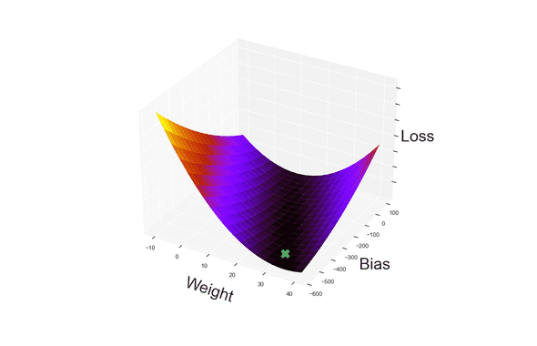
Here y was our loss and x the weight (w). Now, we need another dimension for the bias b since the loss of our model depends on the values we’ll set for w and b.

That means our loss function has three axes and might look like the following with some random values for the weight and bias. The green cross indicates the graph’s minimum.

In our scenario, where we have a function like this, which depends on two input parameters x,y aka w,b, the Gradient is a vector that can be interpreted as the “direction and rate of fastest increase”. In other words: it shows the direction of steepest ascent from a given position in our graph.

Imagine you’re standing in the valley of a mountain and you’re pointing to the top of the mountain with your finger. Your finger is in this case the Gradient. It points to the steepest ascent.

And the opposite of this direction is the one of the steepest descent. What happens if we follow this direction? We reach the graph’s minimum. The spot where our loss is the smallest for a given w and b. Using the coordinates at this position for the weight and bias will our model make the best predictions.

How do we calculate the Gradient when the function has two parameters? Just as above, we calculate the partial derivatives with respect to x (weight). Additionally, we do the same with respect to y (bias).

Let’s implement this in Python. We can take over the partial derivatives we calculated more above for w. Moreover, we don’t pass 0 as argument anymore when calling predict(), but b.

# The partial derivatives of "loss" with respect to w and b
def gradient(X, Y, w, b):
    w_gradient = 2 * np.mean((predict(X, w, b) - Y) * X)
    b_gradient = 2 * np.mean((predict(X, w, b) - Y) * 1)
    return (w_gradient, b_gradient)

Keep in mind, that the Gradient is a vector. In this case a vector with two elements. That’s why we’re returning two values from gradient().

Since we have two Gradients from now on, we have to change our train() function. Both values w and b must be updated after each iteration.

# Train the model using Gradient Descents algorithm
def train(X, Y, iterations, lr):
    w = b = 0 # Initial weight and bias

    # Gradient Descents iterations
    for i in range(iterations):
        w_gradient, b_gradient = gradient(X, Y, w, b)
        w -= w_gradient * lr
        b -= b_gradient * lr
    return w, b

The prediction

Finally, we have everything we need to answer the question from the beginning. This is our codebase:

# The model's output (prediction)
def predict(X, w, b):
    return X * w + b

# Calculating the loss using MSE
def loss(X, Y, w, b):
    return np.mean((predict(X, w, b) - Y) ** 2)

# The partial derivatives of "loss" with respect to w and b
def gradient(X, Y, w, b):
    w_gradient = 2 * np.mean((predict(X, w, b) - Y) * X)
    b_gradient = 2 * np.mean((predict(X, w, b) - Y) * 1)
    return (w_gradient, b_gradient)

# Train the model using Gradient Descents algorithm
def train(X, Y, iterations, lr):
    w = b = 0 # Initial weight and bias

    # Gradient Descents iterations
    for i in range(iterations):
        w_gradient, b_gradient = gradient(X, Y, w, b)
        w -= w_gradient * lr
        b -= b_gradient * lr
    return w, b

Well, what was the question again?

How many visitors can we expect to see in our park tomorrow when know that there will be 33°C at this day?

1. Read the training data
2. Train the model
3. Make the prediction
4. Output

# Load training data into Numpy array
X, Y = np.loadtxt("park.txt", skiprows=1, unpack=True)

# Train the model
w, b, loss_values = train(X, Y, iterations=20000, lr=0.001)

# Output
print("\nw=%.8f; b=%.8f" % (w, b))
print("Prediction: x=%d => y=%.2f" % (33, predict(33, w, b)))

When our model has finished its training it will set proper values for w and b. Now we can use those two parameters and predict the output for x = 33. We simply call predict() and pass in the according arguments.

When we run the Python programm and predict the value we’ll get the following output for the weight, bias and the prediction:

As you can see we can expect ~543 visitors for the next day. We’re also able to predict the number of visitors for any other day. We just have to change the X parameter (degrees) we pass in when calling predict().

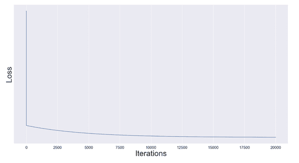
Let’s have a look on how the model improved after each iteration of the trainings phase. Did it improve at all?

As you can see the loss was very high at the beginning. That’s where the model was the worst but improved the fastest. Afterwards, the improvement became less and less after each iteration. At the end the loss decreased slower since the Gradients decreased.

Remember the linear function from the beginning that describes our model? This function looks as follows now:

It is used to predict values. It’s the heart of our machine learning model. The cool thing here is that the machine learned by itself to set proper values for x and y with the help of the training data from the beginning. Magic!

That’s it! I hope this article helped you to better understand Gradient Descent in Python. You can find the complete source code at GitHub with some extra functions to create the diagrams from this article.

The code and my knowledge is mostly based on the book ”Programming Machine Learning” by Paolo Perrotta. You should definitely check it out.