Recognizing hand drawn Doodles using Deep Learning

In November 2016 Google released an online game called ”Quick, Draw!” that asks the player to draw an image of a prescribed object and then uses a neural network to guess what the drawing represents. All in all there are 345 different objects the neural network can recognize.

Luckily, Google released the dataset they trained their neural network with, which includes more than 50 million by the players hand drawn images. So you can use this dataset to train your own neural network. And that’s exactly what this article is about: we’ll build a convolutional neural network to recognize hand drawn images using the Quick, Draw! dataset. Furthermore, we’ll build a simple web app that allows the user to draw images and predict them using the network model later on.

The complete code and the trained model are available at GitHub. You can find the webapp demo on Fly.io.

Neural Network

What we’ll do:

1. Generate, load & visualize the training data
2. Design the network
3. Train & export the model
4. Convert the model to TFLite

Setup

For developing the convolutional neural network we’ll use the following dependencies as listed in requirements.txt:

tensorflow==2.6.2
numpy~=1.19.5
quickdraw==0.2.0
matplotlib==3.3.4
jupyter==1.0.0
pillow==8.4.0

Tip: create a new virtual environment for that.

Install the dependencies using the following command.

pip3 install -r requirements.txt

Let’s have a look at the dataset before writing the actual code.

Dataset

You can find the complete dataset at Google Cloud Platform, which contains more than 50 million images of 345 different categories. A list of all included categories is avaiable here.

A single image is represented as follows in the Quick, Draw! dataset:

{
  "key_id":"5891796615823360",
  "word":"nose",
  "countrycode":"AE",
  "timestamp":"2017-03-01 20:41:36.70725 UTC",
  "recognized":true,
  "drawing":[[[129,128,129,129,130,130,131,132,132,133,133,133,133,...]]]
}

The following properties are important for us:

• word (the image’s category)
• recognized (whether the drawing was recognized by Google’s AI)
• drawing (an array representing the vector drawing)

The actual image in “drawing” is a multi-dimensional array including the pixel coordinates of each single stroke:

[
  [  // First stroke
    [x0, x1, x2, x3, ...],
    [y0, y1, y2, y3, ...],
    [t0, t1, t2, t3, ...]
  ],
  [  // Second stroke
    [x0, x1, x2, x3, ...],
    [y0, y1, y2, y3, ...],
    [t0, t1, t2, t3, ...]
  ],
  ... // Additional strokes
]

Generation

In order to train the neural network we create our own slightly modified dataset from Google’s one. For downloading and accessing the one from Google Cloud Platform we use a Python package called quickdraw.

The following steps are required to create our own dataset:

1. Load 1200 training images for each class from the cloud storage
2. Resize them to 28x28 pixels
3. Save them as PNG

image_size = (28, 28)

def generate_class_images(name, max_drawings, recognized):
    directory = Path("dataset/" + name)

    if not directory.exists():
        directory.mkdir(parents=True)

    images = QuickDrawDataGroup(name, max_drawings=max_drawings, recognized=recognized)
    for img in images.drawings:
        filename = directory.as_posix() + "/" + str(img.key_id) + ".png"
        img.get_image(stroke_width=3).resize(image_size).save(filename)

for label in QuickDrawData().drawing_names:
    generate_class_images(label, max_drawings=1200, recognized=True)

Setting recognized=True ensures that only images that have been recognized by Google’s AI are loaded.

After the generation is finished there should be a directory structure that looks like the following. Each class has its own subdirectory including 1200 images:

.
└── dataset
|   ├── aircraft carrier
|   │   ├── 4504134474530816.png
|   │   ├── 4506833509154816.png
|   │   ├── ...
|   ├── airplane
|   │   ├── 4508382553702400.png
|   │   ├── 4508818253807616.png
|   │   ├── ...
|   ├── ...

In total there should be 414.000 images (345 * 1200).

Loading

Now we can load the images using Keras image_dataset_from_directory function and split them into a training and validation set. The batch size is set to 32.

batch_size = 32

train_ds = image_dataset_from_directory(
    dataset_dir,
    validation_split=0.2,
    subset="training",
    seed=123,
    color_mode="grayscale",
    image_size=image_size,
    batch_size=batch_size
)

val_ds = image_dataset_from_directory(
    dataset_dir,
    validation_split=0.2,
    subset="validation",
    seed=123,
    color_mode="grayscale",
    image_size=image_size,
    batch_size=batch_size
)

Using a 80/20 split we end up having 331.200 training and 82.800 validation images.

Visualization

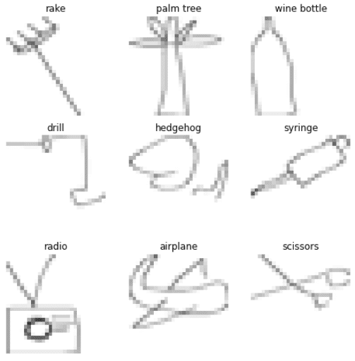
Next, let’s visualize some random training images using matplotlib:

plt.figure(figsize=(8, 8))
for images, labels in train_ds.take(1):
    for i in range(9):
        ax = plt.subplot(3, 3, i + 1)
        data = images[i].numpy().astype("uint8")
        plt.imshow(data, cmap='gray', vmin=0, vmax=255)
        plt.title(train_ds.class_names[labels[i]])
        plt.axis("off")

What outputs:

Architecture

In the next step we design the convolutional neural network. Therefore, we make use of the following 7 Keras layers:

• Rescaling
• BatchNormalization
• Conv2D
• MaxPooling2D
• Flatten
• Dense
• Dropout

There are 345 classes in total. The input shape is (28, 28, 1) since all images have a size of 28x28 pixel and 1 color channel (grayscale).

n_classes = 345
input_shape = (28, 28, 1)

model = Sequential([
    Rescaling(1. / 255, input_shape=input_shape),
    BatchNormalization(),

    Conv2D(6, kernel_size=(3, 3), padding="same", activation="relu"),
    Conv2D(8, kernel_size=(3, 3), padding="same", activation="relu"),
    Conv2D(10, kernel_size=(3, 3), padding="same", activation="relu"),
    BatchNormalization(),
    MaxPooling2D(pool_size=(2, 2)),

    Flatten(),

    Dense(700, activation="relu"),
    BatchNormalization(),
    Dropout(0.2),

    Dense(500, activation="relu"),
    BatchNormalization(),
    Dropout(0.2),

    Dense(400, activation="relu"),
    Dropout(0.2),

    Dense(n_classes, activation="softmax")
])

Moreover, here’s a summary of the model. In total the modal has 2,068,019 parameters. 2,065,597 of them are trainable.

Layer (type)                 Output Shape              Param #
=================================================================
rescaling (Rescaling)        (None, 28, 28, 1)         0
_________________________________________________________________
batch_normalization (BatchNo (None, 28, 28, 1)         4
_________________________________________________________________
conv2d (Conv2D)              (None, 28, 28, 6)         60
_________________________________________________________________
conv2d_1 (Conv2D)            (None, 28, 28, 8)         440
_________________________________________________________________
conv2d_2 (Conv2D)            (None, 28, 28, 10)        730
_________________________________________________________________
batch_normalization_1 (Batch (None, 28, 28, 10)        40
_________________________________________________________________
max_pooling2d (MaxPooling2D) (None, 14, 14, 10)        0
_________________________________________________________________
flatten (Flatten)            (None, 1960)              0
_________________________________________________________________
dense (Dense)                (None, 700)               1372700
_________________________________________________________________
batch_normalization_2 (Batch (None, 700)               2800
_________________________________________________________________
dropout (Dropout)            (None, 700)               0
_________________________________________________________________
dense_1 (Dense)              (None, 500)               350500
_________________________________________________________________
batch_normalization_3 (Batch (None, 500)               2000
_________________________________________________________________
dropout_1 (Dropout)          (None, 500)               0
_________________________________________________________________
dense_2 (Dense)              (None, 400)               200400
_________________________________________________________________
dropout_2 (Dropout)          (None, 400)               0
_________________________________________________________________
dense_3 (Dense)              (None, 345)               138345
=================================================================
Total params: 2,068,019
Trainable params: 2,065,597
Non-trainable params: 2,422

Training

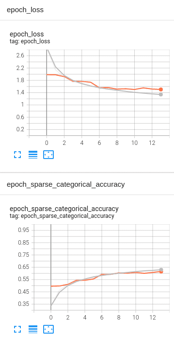
We’ll train the neural network for 14 epochs. At the end of the training the resulting Keras model is saved to the models directory. Additionally, TensorBoard helps us to visualize the training process.

epochs = 14

logdir = os.path.join("logs", datetime.datetime.now().strftime("%Y%m%d-%H%M%S"))
tensorboard_callback = TensorBoard(logdir, histogram_freq=1)

model.fit(
    train_ds,
    validation_data=val_ds,
    epochs=epochs,
    verbose=1,
    callbacks=[tensorboard_callback]
)

model.save('./models/model_' + datetime.datetime.now().strftime("%Y%m%d-%H%M%S"))

After 14 epochs of training the network has a validation accuracy of 61.15%, what’s not that bad for 345 categories. Especially because there a similarities between some. I’m sure there are still some things you can improve to get an even better score.

Export

Last but not least since the web application requires a TFLite model, we have to convert the Keras model as described here.

# Convert the model
converter = tf.lite.TFLiteConverter.from_saved_model("models/<Model>") # path to the SavedModel directory
tflite_model = converter.convert()

# Save the model.
with open('model.tflite', 'wb') as f:
  f.write(tflite_model)

Web-App

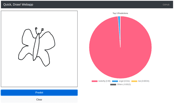
Next we’ll create the web application which is a simple FastApi server that hosts a single static HTML page where the user can draw a canvas and the predicted labels are output as a pie chart with their probabilities. The REST API includes a single POST endpoint which is used for transforming the canvas.

Make sure to checkout the live demo.

Setup

For developing the web application we’ll use the following dependencies as listed in requirements.txt:

fastapi==0.71.0
Pillow==9.0.0
starlette==0.17.1
uvicorn==0.16.0
gunicorn==20.1.0

Backend

The backend is required to resize the canvas to 28x28 pixel as our training images and to crop its content square and remove blank space.

Instead of using Python you can accomplish the same using Tensorflow’s resizeBilinear function. However, I have had bad experiences with this function. Using it causes a huge quality loss of the image with unwanted color effects. That’s the reason why I’m using Pillow on the backend side.

The endpoint /transform expects an image’s strokes and the bounding box for cropping it. Using these two parameters we call transform_img which draws the image using it strokes, resize it and crops it. The resulting image is returned from the endpoint.

class ImageData(BaseModel):
    strokes: list
    box: list

app = FastAPI()

@app.post("/transform")
async def transform(image_data: ImageData):
    filepath = "./images/" + str(uuid4()) + ".png"
    img = transform_img(image_data.strokes, image_data.box)
    img.save(filepath)

    return FileResponse(filepath, background=BackgroundTask(remove, path=filepath))

app.mount("/", StaticFiles(directory="static", html=True), name="static")

def transform_img(strokes, box):
    # Calc cropped image size
    width = box[2] - box[0]
    height = box[3] - box[1]

    image = Image.new("RGB", (width, height), color=(255, 255, 255))
    image_draw = ImageDraw.Draw(image)

    for stroke in strokes:
        positions = []
        for i in range(0, len(stroke[0])):
            positions.append((stroke[0][i], stroke[1][i]))
        image_draw.line(positions, fill=(0, 0, 0), width=3)

    return image.resize(size=(28, 28))

The final image looks as follows:

It has a resolution of 28x28 pixel and it’s cropped.

Frontend

Let’s continue with the frontend part of our web application. Here, we’ll need a drawing area which allows the user to draw a canvas. p5.js is a great library for such a use case.

NOTE: I will not cover each line of code here, only the important ones. As I mentioned above you can finde the complete code here.

Model & Labels

First of all, we load our previous trained TFLite model using tfjs:

const loadModel = async () => {
  console.log("Model loading...")

  model = await tflite.loadTFLiteModel("./models/model.tflite")
  model.predict(tf.zeros([1, 28, 28, 1])) // warmup

  console.log(`Model loaded! (${LABELS.length} classes)`)
}

LABELS is an array that contains all 345 image categories. For reasons of space I placed them in a separate file. The order of the its elements is really important, don’t change it! Otherwise your model will make wrong predictions.

Drawing

Setup p5.js as follows:

const WIDTH = 500
const HEIGHT = 500
const STROKE_WEIGHT = 3

function setup() {
  createCanvas(WIDTH, HEIGHT)
  strokeWeight(STROKE_WEIGHT)
  stroke("black")
  background("#FFFFFF")
}

Handling mouse movement and click inside the canvas:

function mouseDown() {
  clicked = true
  mousePosition = [mouseX, mouseY]
}

// Check whether mouse position is within canvas
function mouseMoved() {
  if (clicked && inRange(mouseX, 0, WIDTH) && inRange(mouseY, 0, HEIGHT)) {
    strokePixels[0].push(Math.floor(mouseX))
    strokePixels[1].push(Math.floor(mouseY))

    line(mouseX, mouseY, mousePosition[0], mousePosition[1])
    mousePosition = [mouseX, mouseY]
  }
}

function mouseReleased() {
  if (strokePixels[0].length) {
    imageStrokes.push(strokePixels)
    strokePixels = [[], []]
  }
  clicked = false
}

When the mouse is clicked and moved its x/y coordinates are collected in strokePixels. So the array contains all x and y pixels of the current drawn stroke:

[
  [x1, x2, ..., xn],
  [y1, y2, ..., yn]
]

When the mouse is released, the “current stroke” is finished and added to the imageStrokes array which contains all drawn strokes of the canvas. In fact it’s an array of strokePixels:

[
  // First stroke
  [[x0, x1, x2, x3, ...], [y0, y1, y2, y3, ...]],

  // Second stroke
  [[x0, x1, x2, x3, ...], [y0, y1, y2, y3, ...]],
  ...
]

Preprocessing

Before predicting the label we have to preprocess the canvas using our /transform endpoint and Tensorflow.js. Therefore, we use the imageStrokes array that contains all the canvas’ strokes:

const preprocess = async cb => {
  const { min, max } = getBoundingBox()

  // Resize to 28x28 pixel & crop
  const imageBlob = await fetch("/transform", {
    method: "POST",
    headers: {
      "Content-Type": "application/json",
    },
    redirect: "follow",
    referrerPolicy: "no-referrer",
    body: JSON.stringify({
      strokes: imageStrokes,
      box: [min.x, min.y, max.x, max.y],
    }),
  }).then(response => response.blob())

  const img = new Image(28, 28)
  img.src = URL.createObjectURL(imageBlob)

  img.onload = () => {
    const tensor = tf.tidy(() =>
      tf.browser
        .fromPixels(img, 1)
        .toFloat()
        .expandDims(0)
    )
    cb(tensor)
  }
}

The function getBoundingBox calculates the minimum / maximum x and y coordinates of the drawing inside the canvas. Those values are used to crop the canvas on the backend side and remove the white background.

Prediction

When making predictions we use our model and the tensor returned from preprocess. Afterwards, we select the top 3 predictions and output their probabilities with a pie chart.

const predict = async () => {
  if (!imageStrokes.length) return
  if (!LABELS.length) throw new Error("No labels found!")

  preprocess(tensor => {
    const predictions = model.predict(tensor).dataSync()

    const top3 = Array.from(predictions)
      .map((p, i) => ({
        probability: p,
        className: LABELS[i],
        index: i,
      }))
      .sort((a, b) => b.probability - a.probability)
      .slice(0, 3)

    drawPie(top3)
    console.log(top3)
  })
}

That’s it! You just created an application that recognizes hand drawn images using Deep Learning. Show the app to your friends and family. I’m sure they’ll be quite impressed.